Suppose you are going on vacation and you realise you need a new suitcase. So you quickly head to your e-commerce app of choice and type the query “suitcase”. Or…. should the query rather be “luggage”? Or “travel bag”?
Ideally, it should not matter – you should not need to think about how you phrase your query. As long as you express your buying intention, you should get approximately the same set of results in your search regardless of the exact words you used.
For a long time, that was not the case in e-commerce search engines, as they relied heavily on lexical search. In its vanilla form, this approach matches exact words in users’ queries to words in product metadata. While fast and effective, lexical search has an important limitation, known in the literature as the “vocabulary gap”. Essentially, it fails to account for synonyms, related concepts or semantic meaning, which can lead to a recall problem: relevant products are not retrieved in user’s search results, despite being relevant. This is illustrated in Figure 1.

To solve this problem, we decided to build a semantic model in order to complement our already existing lexical search at eMAG.
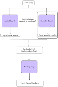
Before delving into the model itself, we briefly describe the larger picture of our search system (Figure 2), in order to understand where this model fits in.
Typically, search comprises two stages: retrieval and ranking. In retrieval, the goal is to resurface the few relevant (or potentially relevant) products to the query, out of the entire catalogue. The second stage of ranking reorders the products retrieved in order to display the most relevant products first. Because only a small fraction of products need to be ranked, ranking can be more resource-intensive, while retrieval needs to be very fast.
The semantic model we set out to build is part of the retrieval stage. As the
image shows, when a search query is issued, it is simultaneously run through both lexical and semantic engines. Each engine returns its set of top results, which are later merged and ranked.
In this post, we will focus solely on explaining the semantic model.
Our challenge ahead was not straightforward, as the main language of our product catalogue and search queries is Romanian, which is a far less resourced language than English.
To begin with, we evaluated two baseline solutions: using an off-the-shelf, small, English-pretrained model and a high-performing embedding model behind an API. We evaluated both solutions on our in-house relevance evaluation dataset: the pretrained model performance was rather low, while the model behind the API achieved a significantly higher performance. As a result, we set ourselves the goal of fine-tuning the model on our data, aiming for performance comparable to that of the API model.
To achieve that, we first needed to build a relevance dataset for training.
Building our relevance dataset with LLMs
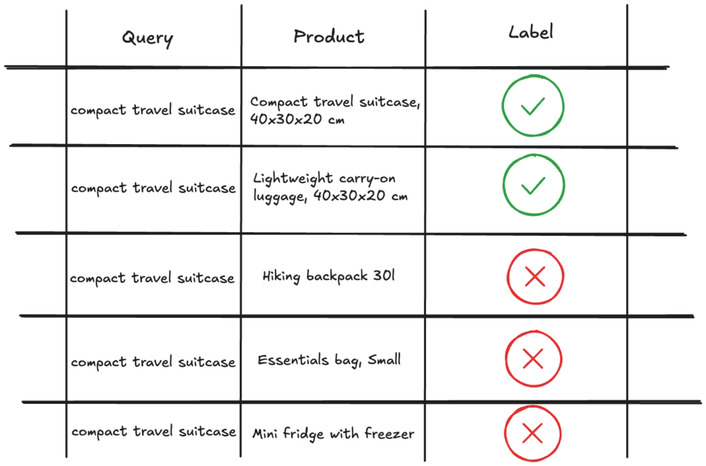
A relevance dataset consists of annotated query-product pairs, also called relevance judgements, where the label denotes whether the product is relevant to the query or not. The notion of relevance is subjective, and it also depends on the task at hand. For our task, we proceeded with binary labels, as follows:
- “relevant” implies the product is an exact match to the query and fulfils all query specifications (i.e. “external ssd samsung 1TB ” is an exact match for the query “portable ssd 1TB”)
- “irrelevant” covers for all other cases, whether the product in question is related (i.e. “external hdd 500GB”), complementary (i.e. “portable ssd case”), or completely irrelevant (i.e. “desk lamp”)
The goal of this dataset is to teach the model to discriminate, given a query, between relevant and irrelevant products (referred to as positive and negative products, respectively).
Traditionally, there were two approaches to building a relevance dataset. One approach consists of deriving relevance judgements implicitly from traffic logs. While cheap and abundant, traffic logs are noisy and suffer from multiple biases. Moreover, they can perpetuate the status quo – for example, if some queries have low recall, many relevant products will not be part of traffic logs and will therefore be omitted from future training data. The other approach entails assigning annotators to label query-product pairs – this method produces higher accuracy data, but it is much more expensive.
For this task, we decided to experiment with generating a dataset labelled by LLM’s, since existing literature reported promising results.
We first created a golden dataset with labelled query-product pairs, which helped us choose an LLM-based judging mechanism.
Afterwards, we proceeded with choosing the query-product pairs to be labelled by the LLM. We sampled the queries in a stratified manner to include queries of various popularity and spanning all departments in eMAG (Fashion, Electronics, Home, Consummables, etc). Then, for each query, we sampled a set of products retrieved from multiple search systems. Utilising multiple search systems meant that we had a wider coverage of products, and we included items that would not have been otherwise recalled. Given the chosen pairs, we labelled them with the selected LLM-based judging mechanism and obtained a mix of positive and negative query-product pairs.
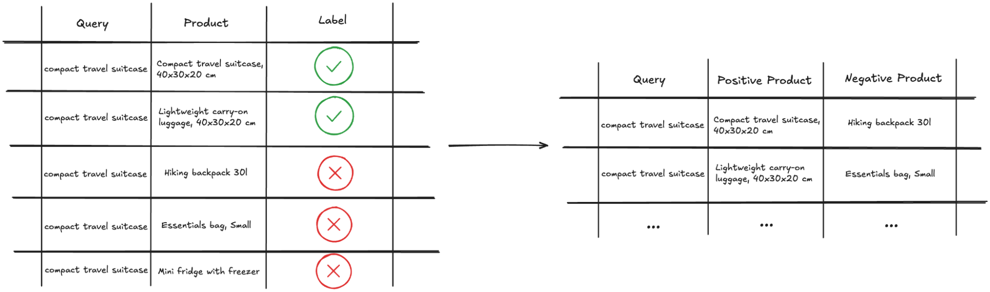
Finally, we increased the diversity of our dataset by further augmenting with negative products from multiple sources:
- categories similar to the categories where positive products were found (i.e. “backpack” for the query “travel bag”)
- categories semantically far from the ones where positive products were found (i.e. “tv” for the query “travel bag”)
This approach allowed us to create a parameterizable blend of easy negatives (products that are clearly not suited for the query) and hard negatives (products that are more difficult to differentiate from positive examples). As we will discuss later, this strategy is recommended in the literature for model training and has also led to significant improvements in our results.
The final dataset is illustrated in Figure 3.
Building our Semantic Model
In developing our model, we explored various architectural options, focusing on cross-encoders and bi-encoders. Cross-encoders generally excel in accuracy but are less practical. Since they combine queries and product representations as a single input to compute a matching score, this process is expected to be applied for each unique query-candidate product pair at query time. That leads to a significantly higher computational load per query and an increased inference time. Conversely, bi-encoders, while less accurate, offer significant speed advantages in retrieval scenarios. This is because only the query needs to be embedded at query time, while document embeddings are precomputed at index time. Given these considerations, we opted for a bi-encoder architecture.
Additionally, due to the hardware limitations of our inference engine, we chose a small-sized English pretrained model for our architecture backbone.
To begin with, we implemented an architecture inspired by the sentence-transformers paradigm, designing a three-tower structure as shown in Figure 4. Queries act as anchors while the other two towers contain positive and negative product representations, respectively.
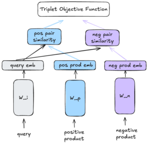
Even though the picture depicts three towers and the model is trained as such, in reality, the weights are shared. This design choice means that once training is complete, any of these towers can function as encoders, capable of processing either queries or product representations and returning vector embeddings. (Figure 5)
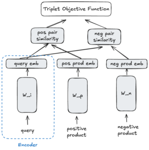
For optimization, we employ a triplet loss function aimed at bringing queries and positive products closer together than queries and negative products. To that goal, we reassembled our dataset of query-product pairs into triplets, where each anchor query had a positive product and a negative product, respectively. (Figure 6)
Semantic search in production
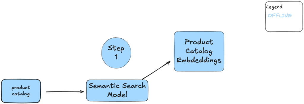
Having trained the model, it is now time to look into how we actually use it. For a better understanding of the benefits given by the bi-encoder architecture, we will explain how the model is used in production, split into two steps.
The first step involves indexing the products. Each product in our catalog is embedded using the Semantic Search Model and further stored in a product index (Product Catalog Embeddings). This offline process ensures that, given no changes in the product metadata, there is no need to repeat this step.
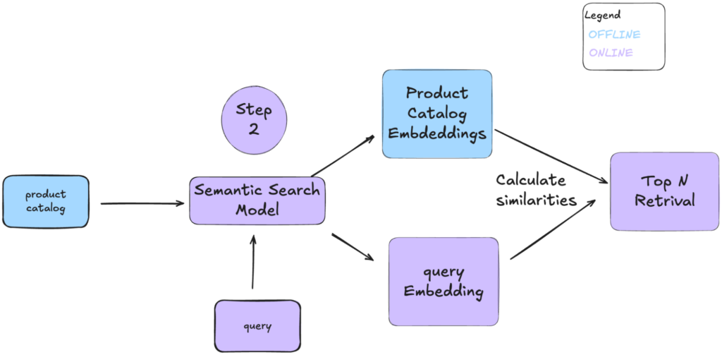
In the online phase (Step 2), incoming queries are embedded using our semantic model. The system then calculates similarities between the query embeddings and the pre-indexed product embeddings, retrieving the top N results. This way, we obtain a beneficial trade-off between relevant retrieved products and short query inference time.
Milestones and Learnings
Our journey in developing this semantic model has been filled with milestones and valuable learnings. While the path was not always smooth, each challenge provided insights that shaped our approach.
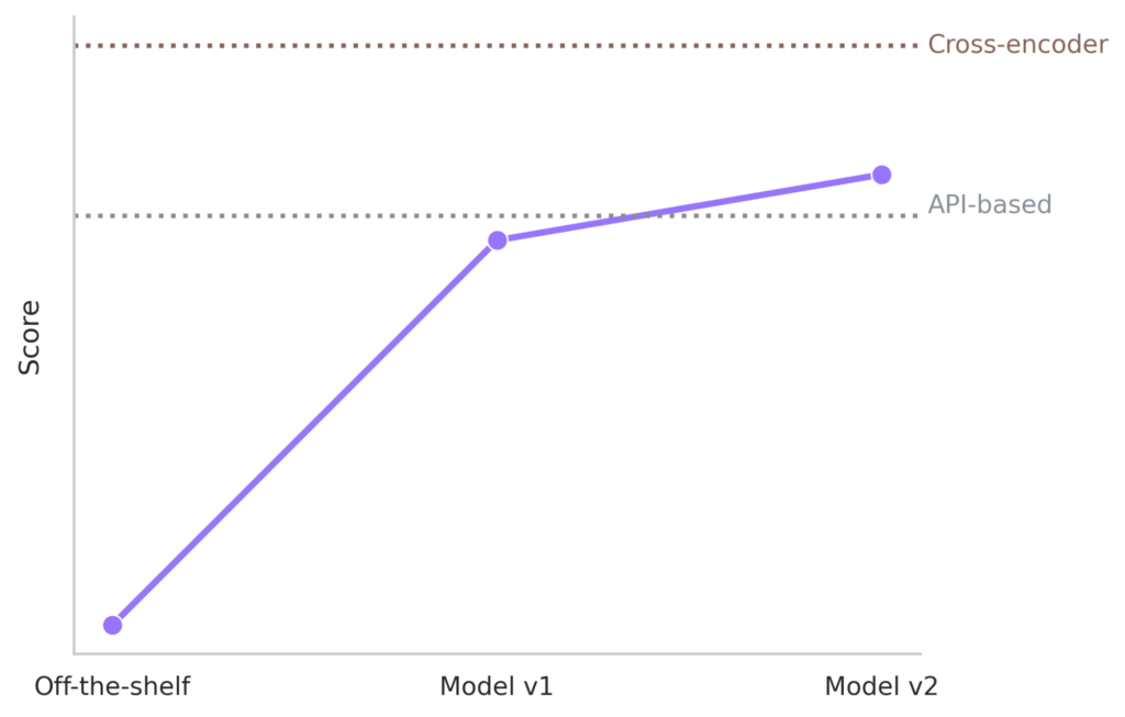
As mentioned before, we set our sights on achieving a performance comparable to API model based embeddings. Moreover, we set a theoretical top-line based on a cross-encoder architecture trained on the same data. Our continuous developments led us to two main versions described below and depicted in Figure 9.
Model v1 was developed by fine-tuning a small, pretrained English language model, and it had a performance that nearly matched that of the API-based solution. Its inference speed was fast, given the relatively small number of parameters.
The next version, Model v2, was built upon a medium-sized multilingual language model and fine-tuned with more in-house data. It reached a performance level that was significantly higher than our initial topline, although clearly below the theoretical topline achieved by the cross-encoder. After distillation, its inference speed was almost as fast as V1. Note that, at the moment of writing, this model is not yet in production.
This progress underscores the importance of continuous iteration and improvement.
Throughout this journey, we’ve gathered several insights:
LLMs as Reliable Annotators: Initially sceptical, we found that large language models (LLMs) can reliably label datasets, enhancing the quality of our training data.
Semantic Search Limitations: While powerful, semantic search is not a one-size-fits-all solution. For certain queries, such as those involving product codes, lexical search still outperforms semantic methods.
Experimentation is Key: There is no universal recipe for success. Experimenting with different blends of easy and hard negatives in the training dataset can yield significant improvements. In this aspect, our findings align with the literature: easy negatives help with model convergence while hard negatives improve representation learning. Because of this, data diversity often trumps sheer data size.
Start Small, Scale Gradually: Model performance does not scale linearly with size. Starting with smaller, more manageable models allows for better control and understanding before scaling up, especially when considering hardware constraints.
Language Considerations: Smaller models may not be trained on less popular languages. It’s crucial to seek alternatives that cater to specific linguistic needs.
Acknowledgements
This work reflects the joint efforts of many teams that are contributing to the eMAG Search project spanning Engineering, Machine Learning, and Product. We would like to thank them all for their involvement in this journey.
If you’re interested in joining our group, check out our careers page.